Definition of Posterior Belief:

$$Bel(x_t) \equiv P(x_t | z_{1:t}, u_{1:t})$$

1st Assumption: Markovian Property

$$P(x_t | x_{t-1}, z_{1:t-1}, u_{1:t}) = P(x_t | x_{t-1}, u_t)$$

2nd Assumption: Sensor Independent

$$P(z_t | x_t, z_{1:t-1}, u_{1:t}) = P(z_t | x_t)$$

Graphical Model Illustration

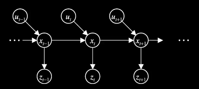
Recursive relationship between $Bel(x_t)$ and $Bel(x_{t-1})$

\begin{equation} \begin{split} Bel(x_t) & = P(x_t | z_{1:t}, u_{1:t}) \\ & = \eta P(z_t | x_t, z_{1:t-1}, u_{1:t})P(x_t | z_{1:t-1}, u_{1:t}) \\ & = \eta P(z_t | x_t)P(x_t | z_{1:t-1}, u_{1:t}) \\ & = \eta P(z_t | x_t)\int P(x_t | x_{t-1}, z_{1:t-1}, u_{1:t})P(x_{t-1} | z_{1:t-1}, u_{1:t})dx_{t-1} \\ & = \eta P(z_t | x_t)\int P(x_t | x_{t-1}, u_t)P(x_{t-1} | z_{1:t-1}, u_{1:t-1})dx_{t-1} \\ & = \eta P(z_t | x_t)\int P(x_t | x_{t-1}, u_t)Bel(x_{t-1})dx_{t-1} \end{split} \end{equation}

Formulation of Kalman Filter¶

$$\text{Objective: } Bel(x_t) = N(\mu_t, \Sigma_t)$$

0th Assumption:

$$Bel(x_0) = N(\mu_0, \Sigma_0)$$

Strong 1st Assumption:

$$x_t = A_t x_{t-1} + B_t u_t + \epsilon_t$$

Strong 2th Assumption:

$$z_t = C_t x_t + \delta_t$$

These assumptions ensure that $Bel(x_t) = N(\mu_t, \Sigma_t)$. The relationship between $\mu_t, \Sigma_t$ and $\mu_{t-1}, \Sigma_{t-1}$ is determined by the following algorithm:

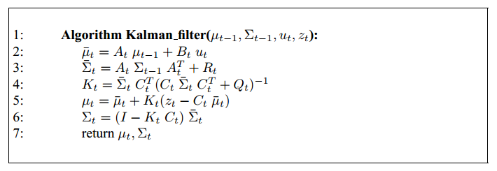
Explanation

$$\text{Prediction} => \int P(x_t | x_{t-1}, u_t)Bel(x_{t-1})dx_{t-1} => \text{line 2, line 3}$$$$\text{Correction} => P(z_t | x_t) => \text{line 5, line 6}$$

Formulation of Particle Filter¶

Particle Filter

$$\text{Objective: } P(x_t \in X_t) \approx Bel(x_t)$$

0th Assumption:

$$P(x_0 \in X_0) \approx Bel(x_0)$$

This assumption, combined with the initial two assumptions of Bayes filter, ensures that the following algorithm will generate the $X_t$ that satisfies $P(x_t \in X_t) \approx Bel(x_t)$:

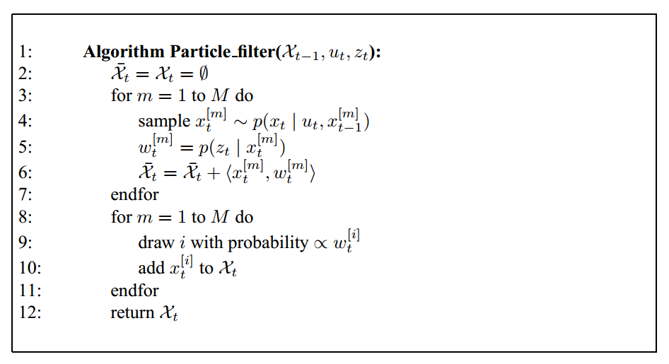
Explanation

$$\text{Prediction} => \int P(x_t | x_{t-1}, u_t)Bel(x_{t-1})dx_{t-1} => \text{line 3, line 4}$$$$\text{Correction} => P(z_t | x_t) => \text{line 9}$$

A Tracking Demo using Particle Filter¶

#%matplotlib inline

import numpy as np
import matplotlib.pyplot as plt
import cv2

from matplotlib import animation, rc
from IPython.display import HTML

fig = plt.figure()
image = None

video = cv2.VideoCapture('images/pres_debate.avi')
window = open("images/pres_debate.txt")
pos   = [int(float(num.strip())) for num in window.readline().split(' ')]
size  = [int(float(num.strip())) for num in window.readline().split(' ')]
template = None

particle_num = 200
particle_set = np.ndarray((particle_num,2), dtype=np.int)
particle_wgt = np.ones((particle_num))

def updatefig(i, *args):
    global image, template, size, pos, window, particle_set, particle_wgt, particle_num
    global l_margin, r_margin, t_margin, b_margin
    ret, frame = video.read()
    
    if ret:
        # Predict next positions
        if template is not None:
            x = particle_set[:,0] + np.transpose(np.random.normal(0.0, 4.0, (particle_num)).astype(np.int))
            y = particle_set[:,1] + np.transpose(np.random.normal(0.0, 4.0, (particle_num)).astype(np.int))
            particle_set[:,0] = np.clip(x, l_margin, r_margin)
            particle_set[:,1] = np.clip(y, t_margin, b_margin)
        else:
            l_margin = int(size[0]/2)+1
            r_margin = frame.shape[1] - int(size[0]/2)-1
            t_margin = int(size[1]/2)+1
            b_margin = frame.shape[0] - int(size[1]/2)-1

            particle_set[:,0] = np.random.randint(l_margin, r_margin, particle_num)
            particle_set[:,1] = np.random.randint(t_margin, b_margin, particle_num)

            template = np.copy(frame[pos[1]:pos[1]+size[1], pos[0]:pos[0]+size[0]])
            template = np.float32(cv2.cvtColor(template, cv2.COLOR_BGR2GRAY))

        # Update particle weights
        for i in range(particle_num):
            x = particle_set[i,0]
            y = particle_set[i,1]
            can_match = np.copy(frame[y-t_margin:y+t_margin-1, x-l_margin:x+l_margin-1])
            can_match = np.float32(cv2.cvtColor(can_match, cv2.COLOR_BGR2GRAY))

            weight = np.exp(-np.sum(np.square(can_match-template))/template.shape[0]/template.shape[1]/2/100)
            particle_wgt[i] = weight
        particle_wgt = particle_wgt/np.sum(particle_wgt)
        
        # Resample the particles
        indices = np.random.choice(particle_num, particle_num, p = list(particle_wgt))
        particle_set = particle_set[indices]

        # Debugging
        for i in range(particle_num):
            cv2.circle(frame, tuple(particle_set[i]), 2, (255,0,0), 2)
    
    if image is not None:
        image.set_array(frame)
    else:
        image = plt.imshow(frame, cmap=plt.get_cmap('hsv'))
        
    return image,

anim = animation.FuncAnimation(fig, updatefig, interval=50, blit=True)

HTML(anim.to_html5_video())

Comments

Object Tracking

Formulation of Kalman Filter¶

Formulation of Particle Filter¶

A Tracking Demo using Particle Filter¶

Published

Category

Tags